Using SPSS for Quantitative Analysis of Complex Data

Mastering tools that simplify and enhance the analytical process of quantitative research data is critical for PhD students. One such tool is IBM SPSS (Statistical Package for the Social Sciences), a versatile software suite tailored for statistical analysis. This blog provides a comprehensive guide on using SPSS for analyzing complex data, from foundational principles to practical applications. For more information and expert assistance with SPSS for your PhD research, get a free consultation from PhD Statistics  and discuss your issues or requirements with a statistical analyst. 

Why SPSS is Ideal for PhD-Level Research

SPSS is an ideal tool for PhD-level research due to its ability to handle diverse datasets and perform sophisticated analyses with ease. Its user-friendly interface combines a spreadsheet-style data editor with intuitive menus and dialogs, making statistical operations accessible even to those without advanced programming skills. This simplicity allows PhD students to focus on interpreting results rather than navigating complex software.

The software supports a comprehensive range of statistical techniques, from basic descriptive statistics to advanced multivariate analyses, catering to the varied needs of PhD research. Additionally, SPSS offers powerful visualization tools for creating professional charts and graphs, essential for presenting findings clearly and effectively. These features enhance the overall quality of research outputs.

SPSS also streamlines the data management process by simplifying tasks like importing, cleaning, and transforming data. Its broad applicability across disciplines, including social sciences, health sciences, business, and education, makes it a versatile choice for PhD scholars.

Setting Up Your Data in SPSS

Before diving into analysis, understanding how to structure and prepare your dataset in SPSS is crucial. This step lays the foundation for accurate and meaningful results.

Data Entry and Import

SPSS supports manual data entry as well as importing data from various formats, including Excel, CSV, and text files. To ensure smooth import:

  • Verify that your data adheres to a rectangular format, with rows representing cases (observations) and columns representing variables.
  • Use consistent variable naming conventions, avoiding spaces or special characters.
  • Ensure that missing data is properly coded (e.g., “NA” or a specific numeric placeholder like -99).

Defining Variables

Each variable in SPSS requires a clear definition:

  • Variable Name: A unique identifier for each variable.
  • Variable Type: Choose from numeric, string, date, or other types based on the data.
  • Variable Labels: Assign descriptive labels to improve readability.
  • Value Labels: Map numeric codes to categorical labels (e.g., 1 = “Male,” 2 = “Female”).

Data Cleaning

Data cleaning ensures the integrity and reliability of your analysis. Common steps include:

  • Identifying and handling missing data.
  • Detecting outliers and deciding whether to retain or exclude them.
  • Checking for duplicates and inconsistencies.
  • Standardizing measurement units and scales where applicable.

Conducting Descriptive Analysis

Descriptive statistics summarize your data, providing insights into its central tendency, variability, and distribution. In SPSS, you can:

  • Use the Descriptive Statistics menu to compute mean, median, mode, standard deviation, and variance.
  • Generate frequency distributions and histograms to visualize data patterns.
  • Employ cross-tabulations to examine relationships between categorical variables.

Example:

Suppose you are analyzing survey data on student satisfaction. Using SPSS, you can compute the average satisfaction score, determine its spread, and visualize the distribution to assess normality.

Advanced Statistical Techniques in SPSS

Once you’ve explored your data using descriptive statistics, you can move on to advanced analyses. Here are some key methods supported by SPSS and their applications:

1. Regression Analysis

Regression analysis explores relationships between dependent and independent variables.

  • Linear Regression: Used for continuous outcomes, such as predicting exam scores based on study hours.
  • Logistic Regression: Suitable for binary outcomes, like modeling the likelihood of passing an exam.

2. ANOVA (Analysis of Variance)

ANOVA tests whether there are significant differences between group means.

  • One-Way ANOVA: Examines differences among groups based on one factor.
  • Two-Way ANOVA: Analyzes the interaction effects of two factors.

3. Factor Analysis

Factor analysis reduces data dimensionality by identifying underlying constructs or “factors.” Commonly used in surveys to validate scales and identify latent variables.

4. Cluster Analysis

Cluster analysis groups cases based on similarities. Useful in market segmentation or categorizing research subjects.

5. Time Series Analysis

Time series analysis examines data points collected over time to identify trends and seasonal patterns. Relevant for longitudinal studies and forecasting models.

Tips for Effective Use of SPSS

To effectively use SPSS in your research, proper planning and preparation are crucial. Begin by clearly defining your research questions and hypotheses to guide your analysis. Familiarize yourself with the statistical methods required for your study, and review SPSS documentation or tutorials to understand the software’s features and capabilities. A solid foundation in both your research design and the tool itself will enhance the efficiency and accuracy of your analysis.

Effective data management is key to leveraging SPSS successfully. Always back up your raw data to safeguard against accidental loss or errors during preprocessing. Use SPSS syntax to document and automate repetitive tasks, ensuring consistency and saving time. Regularly save your work to prevent data loss, especially when handling large datasets or complex analyses.

When interpreting and reporting results, ensure your findings align with your research questions and avoid overgeneralization. Enhance clarity by using visualizations to complement numerical data. Always report effect sizes and confidence intervals alongside p-values for a more nuanced understanding of your results.

SPSS is a powerful ally for PhD students who are working with the complexities of quantitative data analysis. Its intuitive interface, coupled with robust statistical capabilities, allows researchers to derive actionable insights from their data. By following best practices and leveraging the features discussed in this blog, PhD students can confidently tackle the quantitative aspects of their research, ensuring their findings are both rigorous and impactful. Whether you are analyzing survey responses, experimental data, or longitudinal trends, SPSS provides the tools needed to transform raw data into meaningful conclusions. Check out our range of statistical software support for more information regarding how you can utilize PhD Statistics for your research requirements. 

PRISMA Statement – Exploring the PRISMA Flow Diagram

The concept of preferred Reporting Items for Systematic Reviews and Meta Analyses (PRISMA)
statement was first published in the year 2009, with an intent to enhance the clarity,
transparency, quality as well as value of the reports. Since then, it has earned not just
acceptance but become extremely popular in the research and publication of systematic reviews
and Meta Analyses. Most of the reputed journals instruct authors to incorporate in their research
techniques.
PRISMA is a rigorous process which collates all the empirical evidence which is applicable to
the pre-defined set of eligibility criteria. It addresses specific hypothesis. Systematic reviews
benefit the researcher by having the ability to offer clear as well as reliable conclusions so that
vast amount of information can be conveyed and at the same time reduce the introduction of
any kind of bias. In addition to that, meta-analysis offers the opportunity to do a critical
assessment as well as give a comprehensive and clear pool of results which aims to increase
statistical power. The studies involving meta-analysis critically evaluates the comprehensive
pool of results of lot of comparable trials with the intent of statistical power.
Because of the objective to do a comprehensive appraisal, the information being presented is
not just clear but at the same time transparent as well as complete. To ensure this kind of
transparency and the consistency of reports, the Quality of Reporting of Meta Analysis
(QUOROM) guidelines were initially also drafted and later updated by the PRISMA statement.
The complete PRISMA statement consists of a 27-item checklist and a flow diagram in addition
to that. All of this is accessible on its website. The website also has explanatory document
which gives examples from already published work addressing each of the items on the
checklist. Though the checklist isn’t an instrument for quality assessment, it sure is a valuable
template for authors to be able to utilize at the time of systematic reviews, especially the
explanatory document that gives the examples from published work which addresses each of
the items that are there in the items given on the list. Despite the fact that the checklist isn’t an
instrument for quality assessment, it is an extremely important and worthy template for
researchers when applying systematic reviews.
Let us look at the four stages of the PRISMA Flow diagram
The work described in the flow diagram is divided into 4 stages:

  1. Identifying the articles for review
  2. Screening the articles for review
  3. Deciding on the studies’ eligibility
  4. Finalizing the list of studies to include in the systematic review
PRISMA Statement

Applying Likert Scale in Social Sciences Surveys and Applications: Reasons and Advantages

Market research is a dominant component of research in the industry. A key aspect of this research is the ability to understand the opinion of the respondents toward a brand, feature, product, service, or anything else. When a researcher measures the opinions of the respondents, he is also able to analyze and measure the level of changes that are required. The Likert scale is a widely used quantitative data collection tool that is used in the research process. It allowed researchers to understand and quantify the sentiments of the respondents. Most of the research that is taken up by brands can make timely and relevant changes because of being able to quantify emotion or sentiment.

Let us first understand what is Likert Scale

A Likert scale is a unidimensional scale that is used by researchers to collect data about the opinions and attitudes of the respondents. The psychometric scale was often used by researchers to get a hang of the views and perspectives of a brand, its product, or its target market.

There are many scales that are available which are directly focused on measuring the opinion of the people. Some of them are Guttman Scale, Bogardus Scale, and Thurstone Scale.

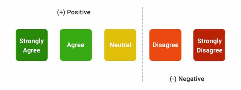
Example of a Likert Scale:

A researcher can apply the Likert scale question to get a response on the feedback of a product as a dichotomous option.  The researcher will frame the question as a statement and not in question firm, such as:” The quality of the product was satisfactory”. The options listed will agree or disagree. Another way to frame the same statement or question would be, “Mark your level of satisfaction with the quality of the product.” the options given to the respondents can range from dissatisfied to satisfied.

 As a respondent to a question like this, the response will be based explicitly on the agreement or disagreement level and the Likert scale creates the scope for determining the agreement or disagreement of the respondents. The main assumption of the Likert scale is that the strength and the intensity of the experiences are Linear in nature. Hence, it stretches from a complete agreement to a complete disagreement, with an assumption that attitudes can be measured.

Example of a Likert Scale

Variations in Likert Scale

In the field of research, the Likert scale is the most preferred scale used for research related to market study where the responses of the customer have to be collected to assess their satisfaction level, preferences, experiences, etc. The Likert scale can be divided into two major types.

  • Even Likert Scale
  • Odd Likert Scale


  • Even Likert Scale:  The even Likert scale is used when researchers want to collect extreme opinions or feedback from the respondents and not give them any neutral opinions.
  1. Four-point Likert Scale: In this kind of Likert scale, researchers use four extreme options and do not offer any neutral choice to the respondents. Here the various degrees of importance are represented in a four-point Likert scale so it is also called as Four Point Likert Scale of importance.
  2. Eight of recommendation: This is a slight variation of the point Likert Scale: This is also called an eight-point likelihood. This is a slight variation from the four-point Likert scale, where the prominent difference is that the scale has eight options to collect feedback about the likelihood of a recommendation.
  • Odd Likert Scale: The odd Likert Scale is used when the researchers want to give the respondents the option of a neutral response. The variations in this type of Likert scale are
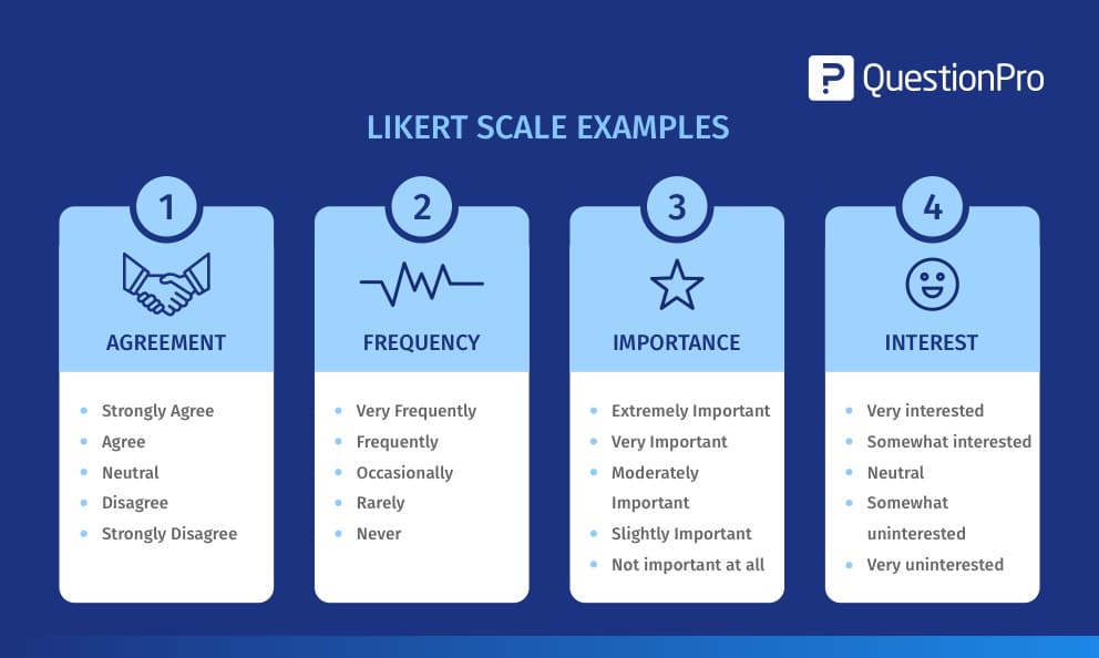
  1. Five Point Likert Scale: with five answer options, researchers use this to gather information about a topic where a neutral response also has relevance or where there may be a possibility that the respondent does not want to answer from the extreme choices given and may want to opt for a neutral response.
  2. Seven-point Likert Scale: This option adds two more answer options at the extreme ends of the 5-point Likert Scale Question
  3. Nine-Point Likert Scale: This kind of Likert scale is not seen much in use and because of the complexity attached to its application, it’s not a preferred option by researchers. It adds two more extreme end options to choose from for the respondent.

Characteristics of Likert Scale

Characteristics of the Likert Scale:

The Likert Scale came into existence in the year 1932 and was first used as a five Point Likert Scale, which is extensively in use even today. These scales range from a group of general topics to more specific ones which can ask respondents on varied topics, ranging from their level of agreement, approval, or belief. Some of the prominent traits or characteristics of the Likert scale are explained here

  • Related Answers: Items should be easily related to the sentence’s answers, regardless of whether the relationship between the item and sentence is evident.
  • Scale Type: There should always be two extreme positions in the items and a middle option which can also be called an intermediate answer which serves as a stepping stone or graduation between the two extremes.
  • The number of options: as stated above, the most common type has been the five-point Likert scale, however as the points are increased from 5 to 7 or 9, the precision in the results also increases. Though this may make the analysis a more complex task to perform the accuracy of the output goes up.
  • Building up the reliability of the scale: Researchers often elongate the ends of the scales and create a seven-point scale. They add a “very” to each of the ends of the scale, that is the top or the bottom. The sever point scale is at the upper limit of the reliability of the scale.
  • Using wide scales: A most common rule recommended by Likert and others is also that, it is better to use a scale that is as wide as possible. At the time of analysis, if required the answers can be collapsed into smaller groups if required.
  • Removing the Neutral response option: a lot of researchers curtail their scale to an even scale and get away with the neutral possibility.   This makes the survey a forced choice survey where the respondent has no choice but to go with one of the extremes as an answer to the statement.
  • Presence of an intrinsic variable:  The application of the Likert scale states that there could be an inherent variable whose values impact the responses or choices made by the respondents in the context of feedback or attitude. This underlying variable is the interval level, best.

Analysis of Likert Scale Data:

Surveys are a common practice with researchers to measure and analyze the quality of products and services. It is a standard classification format for studies. The respondents offer their opinion which is also what makes the data about the quality of a product or service from high to low or better to worse by using points that range from four to nine, depending upon the choice of the researcher taking into consideration various factors. Researchers and auditors generally group collected data into a hierarchy of four fundamental measurement levels – nominal, ordinal, interval, and ratio measurement levels for further analysis:

  1. Nominal Data: This is the kind of data in which the answers when classified into variables will not have quantitative data or a quantifiable order.
  2. Ordinal Data: this kind of data is possible to be classified or sorted but the measurement of the distance between is impossible to do.
  3. Interval data: Interval data is data in which the measurements of the orders and distance are possible to be done.
  4. Ratio Data: this kind of data is quite like interval data. The only difference here is that ratio data has an equal and definite ratio between each data and absolute “zero” is treated as a point of origin.


Data analysis with any of the above four data is straightforward and transparent. The ordinal data analyses, particularly in regards to Likert Scale analyze the data in a more effective manner. This is not a new concern in the field of research. The effectiveness of handling ordinal data as interval data continues to be debatable in survey analysis of various applied fields. 

A few critical points of consideration here are:

  • Statistical Tests: a lot of time researchers treat ordinal data as interval data because it is claimed and preferred that parametric statistical tests are far more powerful than their non-parametric alternatives. To add to it, the inferences that are drawn from parametric tests are easier to interpret and give out more information as compared to their non-parametric counterparts.
  • Focus on the Likert Scale: By just treating ordinal data as interval data, nothing much will be achieved unless the values are examined of the data. Otherwise, the objectives of the analysis can be misled and it can misrepresent the output of the survey. In order to analyze scalar data in a better way, researchers surely consider ordinal data as interval data but also at the same time concentrate on the Likert scale.
  • Checking median or range: the universal guidelines indicate that the mean and standard deviations are not the correct parameters and they are baseless for detailed statistics when the data is on an ordinal scale. This is true for any parametric scale that is based on the normal distribution. The non-parametric is done based on the right median or the range for data inspection.
  • The useful techniques for data analysis: The Likert scale data has the typical characteristics of being discrete, ordinal, and limited in scope.  For a long, there has been a debate and even dispute over the most appropriate way to analyze this data. The first option to be considered is between parametric and non-parametric tests. Let us understand the difference between the use of either of these two tests,
    • Parametric tests assume a regular and uninterrupted division
    • Non-parametric tests do not assume an uninterrupted division. But there is a possibility of concerns about a lesser ability to detect a difference when one of them exists.

Which of these is a better choice to make? Well, the final decision rests in the hands of the researcher and the kind of results that he wants from his study.

Advantages and Disadvantages of the application of the Likert Scale:

The biggest advantage of the Likert Scale is that it is the most universal method for survey collection, therefore they are easy to understand and comprehend. The responses of the Likert scale are easily quantifiable and subjective to the computation of some mathematical analysis. This kind of questionnaire refrains from imposing the respondent to give a simple and concrete yes or no answer and thus does not force him to take a stand on the given statement, especially when the respondent is in any kind of dilemma. It offers the freedom to the respondent to respond in a degree of agreement and this offloads the respondent and puts him in an easier and more comfortable zone. In addition, the Likert scale also creates the scope to accommodate the neutral or undecided feelings of the participants. At the time of coding the responses, the Likert scale responses are the easiest to code as a single number represents the participant’s response.  Over and above the mentioned advantages of the Likert scale in usage and analysis for both the researcher as well as the respondent, these scales are inexpensive, quick, and efficient for data collection. They can be used in a versatile manner and circulated over the internet, given in person, or even sent out by mail for ease with which the respondent can comprehend and respond.

 There are a few disadvantages of this technique, Likert Scale is uni-dimensional in nature and whereas the attitudes of the population for one item in its truest nature exists in a vast and multi-dimensional continuum. The space between the four to nine choices that the Likert scale offers to its respondents cannot be equidistant, as assumed and therefore it fails to measure the accurate attitude of the respondents. In the pattern of a Likert scale questionnaire, the choices of the people are influenced by the previous questions and another big challenge or drawback of this technique is that respondents prefer to go for neutral responses for fear of getting labeled as extremists even though the extreme choices may be more accurate responses. This can impact the authenticity as well as the accuracy of the results.

  • it is not unlikely that peoples’ answers will be influenced by previous questions, or will heavily concentrate on one response side (agree/disagree). Frequently, people avoid choosing the “extreme” options on the scale, because of the negative implications involved with “extremists”, even if an extreme choice would be the most accurate.


The difference between Interaction and Association: Variables as Predictors in a Regression ANOVA Model

It is very common to mix up the concept of association and interaction. Some people also assume that it is imperative for two variables to be associated before they interact. But that is not the truth. When we talk in the context of statistics, these terms have different implications f to signify the relationship between the variables. This becomes all the truer when one is talking about the predictions in the case of the Regression or ANOVA model.
Before we jump to the difference between Association and Interaction, let us briefly but explicitly understand the application of variables in Regression Analysis.
Regression is a statistical technique for finding out the relationship between a single dependent variable which is the criterion and the independent variable which is the predictor. Regression brings forth a predicted value for the criterion aka the dependent variable from a linear combination of the independent variables, aka the predictors. Regression analysis is primarily found to have two uses in the field of scientific literature. One is a prediction along with classification and the other is an explanation
The preliminary step in the regression analysis is to determine the criterion variable. The criterion has acceptable measurement qualities, which are reliability and validity. After having selected the criterion, the predictor variable must be identified. Which is the model selection. The purpose of model selection is to minimize the number of predictors which call for the maximum variance in the criterion. To put it in other words, the most efficient model maximizes the value of the coefficient of determinants. This coefficient estimates the amount of variance in the criterion score that is accounted for by a linear combination of predictor variables. The greater the value of R2, the lesser the error or what we also call the unexplained variance, and hence the better the prediction. R2 is dependent upon the multiple correlation coefficient(R). This does the job of describing the relationship that exists between the expected and the predicted criterion scores, where R equals 1.00. This talks about a perfect prediction where there is not any error and hence no unexplained variance or vice versa. (R2=1.00). In a situation where the value of R is 0.00, there exists no relationship between the predictors and the criterion, and the variance in the scores has also not been explained(R2=0.00). it implies that the chosen variable cannot predict the criterion. The purpose of model selection is, according to what has been stated previously, to build a model that results in the highest estimated value of R2.
According to seasoned researchers, the value of R is often overestimated. The degree of overestimation is often estimated by the sample size. The larger the ratio between the number of predictors ad subjects, the higher the overestimation. To make this better, it is always better to have a large sample size and there should be at least 20-30 subjects allocated to each predictor. The best and most effective way to determine the optimal sample size is through the technique of statistical power analysis.
Another effective way to determine the best model for prediction is to test the significance of adding another variable to the model. This can be done by applying a partial F-Test. The partial F test is like the F test that is used in the analysis of variance. It assesses the statistical significance of the difference between the values for R2 which have been derived from two or more prediction models using a subset of the variables from the main equation.
Though, these above techniques are certainly useful in discussing the most efficient model for prediction. In order to select the right variables, theory must be taken into consideration. Previous literature should be assessed and predictors should be selected for whom the relationship between criterion and predictor has been established.
Assessment of the accuracy of the model is best accomplished by trying to analyze the standard error or estimate also called SEE and further on the percentage of predicted mean represented by SEE(SEE%). The SEE is a representation of the degree to which the predicted scores are deviating from the observed scores on the measure of the criterion. This is quite like the standard deviation that is used in other statistical procedures. Experts suggest that if the values of SEE are lower that means the accuracy of the prediction is more precise. Comparing SEE for different models with the same sample creates room for determining the most accurate model that can be used for prediction. The formula for calculating SEE % is dividing SEE by the mean of the criterion. This can be easily applied to doing a comparison of different models that have been derived from different samples.
The most accurate and efficient model for prediction has been found and it’s advisable to assess the model for stability. One can only call a model stable when it can be applied to diverse samples from the same population and the accuracy of the prediction also does not get diluted. This can be achieved by doing cross-validation of the model. Cross-validation, as the name is suggestive, helps to find out how well the developed prediction model is in another sample that is drawn from the same population. Cross-validation can be done using more than one method. Some of them are using two independent samples, splitting the samples and the PRESS-related statistics that have been developed from the same sample. Let us explore them separately to understand their application.
The use of two independent samples involves the selection of two groups from the same population. The two groups can be classified separately as, the training or exploratory group that is used for establishing the model of prediction. The second group is the confirmatory or validatory group which is used to assess the model for its stability. The experts attempt to compare the R2 value from the two groups and the assessment of “shrinkage”. The difference between the two values of R2 is used as a sign of model stability. Though there is not any specific thumb rule of values to interpret the differences and indicate the stability of a model but expert researchers say that values that are less than 0.10 are indicators of a stable model. One should know that independent samples are used lesser in this context because they greatly impact the cost involved in the research.
The next technique is cross-validation which uses split samples. Once the sample has been chosen from the population, it gets randomly divided into two subgroups. One of the subgroups becomes the group that is called the exploratory sub-group and the other one is termed as the validatory sub-group. Here also the same process is followed and the values of R2 are calculated and the model stability is decided by the calculation of “shrinkage” as discussed above.
The third technique is PRESS-related statistics. It is a solution to the problem of data splitting. This method uses small sample sizes to assess the problem of bias and for the purpose of cross-validation of the model. The trick that is adopted by this technique is to calculate the desired test statistic multiple times and at each attempt, omit individual cases from the calculations. In this method, the difference in the actual values of the criterion for each individual and the predicted value for using the formula derived with the individual’s data removed from the prediction, are calculated. The PRESS statistic is the sum of the squares of the residuals derived from these calculations and is like the sum of squares for the error (SSerror) used in the analysis of variance (ANOVA). The PRESS statistic can be used to calculate a modified form of R2 and the SEE.

What are Association and Interaction and how are they similar and different?
Let us understand what is Association.
The name itself suggests that Association between two variables means that the value of one variable in some way is related to the value of the other variable. The technique for determining this, which is mostly used is by measuring the correlation for two continuous variables and by means of cross-tabulation and a chi-square test for two categorical variables.
Somehow, there is not a very effective measure for the purpose of association between one categorical and one continuous variable Point-biserial correlation works only if the categorical variable is binary. But either one-way analysis of variance or logistic regression can test an association (depending upon whether you think of the categorical variable as the independent or the dependent variable).
Primarily, association means the values of one variable generally co-occur with certain values of the other.
Let us understand what is Interaction.
Interaction is different from Association, even if two variables are associated it says nothing about whether they interact in any way of creating an impact on the third variable. Likewise, if two variables interact, it is possible that they may be associated or not associated.
An interaction between two variables means the effect of one of those variables on a third variable is not constant—the effect differs at different values of the other.
In the case of a Model, what do association and Interaction indicate?
We will try and understand this better with the help of an example. We will have three hypothetical variables, namely, X1, X2, and Y. We will look at three separate situations, in the light of these variables only. X1 will be a continuous variable, X2 a categorical independent variable and Y is a continuous independent variable. This is just one way to categorize them, in another situation, any of these variables could be either categorical or continuous.
Situation 1: Association without Interaction
In this first situation, X1 and X2 are associated. If Y is ignored, the mean of X1 is lowered when X2 =0 than when X2=1. But when it comes to affecting Y, they do not interact. The regression lines become parallel. X1 has the same effect on Y (the slope) for both X2=1 and X2=0.
A simple example is the relationship between height (X1) and weight (Y) in male (X2=1) and female (X2=0) teenagers. There is a relationship between height (X1) and gender (X2). But for both genders, the relationship between height and weight is the same.
This situation can be managed with the help of introducing control variables. Gender is a control variable here, and if that was not introduced, a regression would fit a single line to all these points. It would attribute all the changes in the weight of the respondents to differences in their heights.
Include all the points on a single line, this line would also make the line steeper. Because of this, the unique effect of height on weight would be overestimated.
Situation 2: Interaction without Association
In this second scenario, there is no association between X1 and X2. The mean for X1 remains the same for both categories of X2. But the way in which X1 is affecting Y is different for both the values of X2. This is how one can precisely define Interaction. The slope of X1 on Y is greater for X2=1 than it is for X2=0, in that case, there is no slope at all, and the line is nearly flat.
If we try to look at it as an example, X1 can be the pretest score and Y as the score post-test. Assume that the participants have been randomly assigned to a control(X2=1) or training which is (X2=0).
If the randomization is done fine, the assigned condition which is X2 would not have any relationship with the pretest score which is X1. However, they do have an interaction, the relationship between the pretest and post-test differs in two conditions. In a condition where control exists, without the exposure and effect of training, there would be a high correlation between the pre-test and post-test scores. But in the event where there is exposure to training, if the training does well, the pretest scores would not have much impact on the post-test scores.
Situation 3: Both Interaction and Association
In the third situation, there are both associations and interactions that exist. There is an association between X1 and X2. Again, the mean of X1 is lower in a situation when X2=0 than when X2=1. They also have an interaction with Y. The slopes of the relationship that exists between X1 and Y are different when X2=0 and X2=1. So, X2 has an impact on the relationship between X1 and Y.
A classic example here would be, y can be the number of jobs available in a state and X1 is the eligible workforce that is employable with the degree. X2 is whether the state is rural(X2=0) or Urban(nX2=1).
It is evident and understood that in rural states, the percentage of educated youth as well as job opportunities are lower as compared to urban states. Moreover, in rural regions, there is no relationship between the educational level of the workforce and the number of jobs that are available. It is reversed in the case of urban regions. This situation is also what you would see if the randomization in the last example did not go well or if randomization was not possible.
The distinction between Interaction and Association can become simpler to comprehend as more and more data is analyzed. As researchers, it is suggestive to have a look at your data from the vision of an explorer and use graphs to have a better understanding of what is happening with your variables.

Everything You Need to Know About Mediator and Moderator Variables

Mediator and moderator variables are often used incorrectly or are not given the importance they require in research designs. They serve different functions and are used to explore the causal relationship between independent and dependent variables. This blog deals with their differences and uses in research.

What is a mediator and moderator variable? 

A mediator variable is a variable that plays a role in either the cause or the effect of a studied variable. It is not the sole cause or the main cause, but a variable that plays an important role in the determination of the result. A moderator variable is a variable that either maintains or reduces the influence of the main variable. It can either increase or decrease the variation in the dependent variable. These variables are used to explore the causal relationship between independent and dependent variables. 

Differences in mediator and moderator variables

One of the most common ways to use mediator variables is in bidirectional moderation. In this design, researchers compare the effect of two variables on one another. A good example of this is the study found by Lekach and Banaji on “aging in American culture”. In this study, researchers compare being old to being smart and find that the former has a greater effect on the latter. In this case, the mediator variable is age and the moderator variable is intelligence. By measuring these two variables and seeing which one has the greater effect, researchers can determine why the former has such a larger impact on the latter. Another common approach is to compare two variables in isolation. If researchers want to test the effect of having a child on parents’ satisfaction, they can look at the Big Five Factor of personality and see if having a child has an effect on parents’ satisfaction. 

Implementation of mediator and moderator variables 

There are two basic ways to use mediator and moderator variables in your research.

The first is to use them as independent variables. For example, you could run a study on how having a job affects the stress level of teenagers. You would randomly assign some teens to work and some not to work. Then, you could compare how the teens who were assigned to work compared with the ones who weren’t assigned to work in terms of their stress level.

In this example, your independent variable would be whether or not a teen worked. The dependent variable would be how stressed out that teen was.

The second way is to use them as dependent variables. This means that you use one of these variables in order to predict another variable. For example, let’s say you want to study how having a job affects students’ stress levels. You could randomly assign some students to work and some not to work and then compare their stress levels before and after they got jobs so that you can see if working has any effect on stress levels

Summing up 

There are many ways to use mediation in research and all have their place, but the majority of the time, researchers use them in an integrative fashion. In an integrative design, researchers combine the effects of both variables to determine the overall effect of the study. The most common way to do this is with the mediation model. The mediation model is a statistical tool that can be used to determine if two variables are linked. If they are, researchers can use the variables to make causal claims. However, the model assumes that the dependent variable is influenced by both factors and that these factors are inversely related. If one factor is much higher or lower than the other, researchers will not be able to make causal claims about the relationship between that factor and the dependent variable.