PhD - Statistics Consultation

Exploring Pearson’s Correlation Coefficient Test to Determine Statistical Relationship Between Two Continuous Variables

Scientific research often involves correlation which generally refers to association or any form of link or correspondence. Correlation is nothing but a statistical approach used to evaluate the linear association between two continuous variables. While several types of statistical tests can be deployed to determine the relationship between two quantitative variables, Pearson’s correlation coefficient is considered as the most reliable test used to measure the continuous variables.

Pearson’s correlation coefficient is a statistical test that measures the association or relationship between two continuous variables. Pearson’s correlation coefficient is represented by ‘rho’ and is based on the method of covariance.

The correlation coefficient or ‘rho’ is the slope of regression line between two variables when they have been standardised by subtracting their means & dividing by their standard deviations.

Like any other statistical test, Pearson’s correlation coefficient test has a few assumptions including:

There is a linear relationship between the variables in the sample which can be assessed by plotting the value of variables on a scatter diagram.
The variables must be normally distributed
The variables are either internal or ratio measurements
The outliers must be eliminated completely or kept at minimum
There exists homoscedasticity of data

Properties of the Pearson’s test

Limit – Coefficient values range from -1 to +1, where -1 indicates perfect negative relationship and +1 indicates perfect positive relationship and zero indicates absence of relationship.

Symmetric – Correlation of coefficient between two variables is symmetric which simply means that coefficient value between X and Y or Y and X are symmetric.

Pure number – Pure number is independent of unit of measurement. For instance, if the unit of one variable is in cm and the other is in inches, the Pearson’s correlation coefficient value will remain the same.

When ‘rho’ is utilised as a descriptive statistics, the test doesn’t require any distributional assumptions. When the hypotheses are tested, it is assumed that the observations are independent and variables are distributed on the basis of bi-variate- normal density function.

Testing the hypothesis

Null hypothesis – H0: ρ = 0

Here the population correlation coefficient doesn’t differ significantly from zero. This simply means that there is no significant linear relationship between X and Y.

Alternate hypothesis – Ha: ρ ≠ 0

Here the population correlation coefficient significantly differs from zero. In other words, there is a significant linear relationship between X and Y.

Method 1 – using the P-value to make a decision

If the p-value is less than the significance level, i.e., alpha= 0.05 then reject the null hypothesis. However, there exists evidence to prove the presence of linear relationship between X and Y as the correlation coefficient is significantly different from zero.
If the p-value is equal or greater than the significance level, then the hypothesis shouldn’t be rejected. Here we have sufficient evidence to prove that there is a significant linear relationship

Method 2 – using a table of critical values

95% critical values of the sample correlation coefficient table gives an idea whether the computed value of ‘r’ is significant. The critical value can be found using the degrees of freedom (df=n-2).
If ‘r’ value doesn’t lie between the positive and negative critical values, then the correlation coefficient is considered to be significant.
If ‘r’ is significant, then it can be used for line for prediction. However, if ‘r’ is not significant, then you cannot use the line prediction.

The probability of rejecting a false null hypothesis and probability of type-I error is determined by power and alpha. In Pearson’s correlation coefficient test, the value of power & alpha must lie between zero and one.

Degree of correlation

The major aspect in Pearson’s correlation coefficient test is the value of correlations. Typically, this value lies between -1and 1.

Let’s have a detailed look at various types of correlations depending on their value.

Positive correlations – Here the correlation value is positive and the two variables are perfectly positively related. That is, the dots in a scatter line lie on the straight ascending order.
Negative correlation – In this type of correlation the correlation value is -1 and the data points lie on straight descending order. I.e., the variables are linearly negatively related.
Perfect correlation – The correlation is zero and the variables do not have any linear relationship. However, there is a probability of existence of non-linear relationships.

Besides positive, negative and perfect correlation, depending on the value, we have high. Moderate and low degree correlations.

High degree – Here, the correlation coefficient value lies between ± 0.50 and ± 1.

Moderate degree – The value lies between ± 0.30 and ± 0.49.

Low degree – Here, the value lies below + .29.

A glimpse at an example for the Pearson’s correlation coefficient test

10 students held their breath for a minute after breathing normally for 60 seconds and hyperventilating for 60 seconds. Let’s check if there is any association between the two variables ( normal and hyperventilating breathing) for a minimum of 4 students.

Student	A	B	C	D
Normal breathing	55	55	64	64
Hyperventilating breathing	86	90	84	90

According to the graph, there is a linear relationship between the variables.

Correlation coefficient is one of the most powerful analysis techniques which is purely based on the collected data. Therefore, it is a must to collect accurate data which are capable of providing desired outcomes of the test.

Chi-Square Test: Know about the Inferential Statistical test that Operates on Categorical Variables

Statistical test can be complex but it verifies & assures the quality of the study. In analytical work, the most crucial task is the comparison of data (sets of data) and making interpretations.

Inferential statistics, one among the two major branches of statistics, are concerned with making inferences based on the relationships found in the sample, to that in the population. This kind of statistics back the hypothesis, and such inferential test that supports the existence of group differences in the entire population is the Chi-Square test.

The Chi-Square test assumes (the null hypothesis) that the observed values match the expected values for categorical data. Chi-Square test is of two types,

Chi-Square goodness-of-fit test – This test is performed for one categorical value and begins with hypothesizing that variable distribution behaves in a specific manner. For example, in order to identify the daily staffing needs of a store, the manager would wish to know if there is any consistency in the number of customers throughout the week.
Chi-Square test for independence – This test is conducted for two categorical values. It compares variables in a contingency table & investigates if they are related. However, if the observed data doesn’t fit the model, the likelihood that the variables are dependent enhances, proving that the null hypothesis is incorrect.

For instance, this test can help us determine if the DRE is independent of biopsy results.

Chi-Square goodness-of-fit and test for independence depends only on the degrees of freedom and set of observed and expected values. These tests do not require any assumption pertaining to distribution of the parent population. However, if the test is performed along with the standard approximation, the applicability of Chi-Squared distribution, assumptions such as,

Simple random sample – It is a random sampling from a fixed population where every individual of the distribution/population of sample size has an equal probability of selection.
Constraints on cell frequency must be linear – If a sample with a large size is assumed, but the test is performed on smaller sample size, then the test will yield an inaccurate inference.
Theoretical cell frequency must be greater than 5 – As a rule of thumb, the expected cell count of a 2-by-2 table must be 5 or more and, for larger tables, it must be 5 or 80% of the cells.
Independence of observations – The observations must be independent of each other, which implies that Chi-Square cannot test correlated data such as matched pairs.

Chi-Square statistics

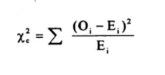
Chi-Square test includes calculating a metric known as Chi-square statistic and the formula used here is,

Chi Square statistic

Where, E=(row total×column total) / sample size

Here the subscript ‘c’ indicates degrees of freedom, ‘O’ is the observed value and ‘E’ is the expected value. The summation indicates that the calculation must be done for each data item in the given data set.

Note that the Chi-square statistic cannot be used for percentages, proportions, and be used only on numbers.

For example, if you have 5% of 100 people, you must first convert 5% into the whole number and then run the test.

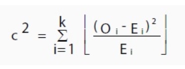
Chi-Square statistic includes variations which utilise the same concept, i.e., comparing observed & expected values. However, the type of variations used depends on how the data was collected and the hypothesis is being tested.

One of the most common forms of variation used for contingency tables is

Chi-Square statistic

Where E is the expected value, O is the observed value, and “i” is the ith position in the contingency table.

How to determine the statistical significance

The low value for Chi-Square implies that the correlation between the two sets of data is high. Theoretically, if the observed & expected values are equal, then Chi-Square would be zero, which is practically impossible.

Determining if the test statistic is large enough to specify a statistically significant difference, includes two processes.

Comparing calculated Chi-Square value and critical value from Chi-Square table. If the Chi-Square value is smaller than that of the critical value, there is no significant difference.
Utilising P-value.

To calculate P-value manually,

Firstly, determine the observed & expected values.
This is followed by calculating the degrees of freedom using the formula,

Degrees of freedom = n-1, where ‘n’ is the number of variables.

Compare observed & expected results with Chi-Square value (using the formula mentioned above).
Choose a significance level (in decimals). Most commonly used value is P=0.05.
Use Chi-Square distribution tables and approximate P value.
Determine whether to reject the null hypothesis or not.

Example of Chi-Square test

Consider a random poll was conducted across 1000 voters (both male & female). The individuals who were classified based on their gender and whether they were supporters of party A, B or C.

	Party A	Party B	Party C	Total
Male	150	200	50	400
Female	270	300	30	600
Total	420	500	80	1000

Calculate the expected value (E) using the above-mentioned formula
In the second step, calculate the Chi-Square statistic
Sum up all the values of Chi-Square statistics results, identify P-value and determine if the result is statistically significant or not

After obtaining the significant result, you can perform follow-up tests such as post-hoc test, to pinpoint the reasons for the significant result. To know more about it, visit https://www.rforge.net/doc/packages/NCStats/chisqPostHoc.html.

Wilcoxon Rank-Sum test : A Non Parametric Alternative to two Sample T-Test

Statistics, a scientific approach to analyzing numerical data, is employed to discover relationships among the phenomena to describe, predict and control their occurrence.

Statistics helps the researcher to acquire precise, steadfast and dependable findings. Although there are several statistical tests such as ANOVA, independent t-test, etc. to arrive at the right result, one must choose the test according to the type of study.

For instance, if one wants to investigate if the means of two or more groups are different from each other, then he/she must use the ANOVA test. On the other hand, if a researcher wants to test the relationship between categorical variables, the Chi-square test is to be used.

Similarly, for the comparison of means of two independent groups, the two-sample t-test is used. However, if the t-test doesn’t satisfy the requirements for two independent samples, then Wilcoxon Rank-Sum is used as it can offer the two independent samples drawn from populations with an ordinal distribution. This test does not assume known distributions, does not deal with parameters, and hence it is considered as a non-parametric test.

Wilcoxon Rank-Sum test also known as Mann-Whitney U test makes two important assumptions. That is the assumption of independence and equal variance. These assumptions are sufficient for determining if the two populations are different. Additionally, if we assume that the two populations are identical (except for a difference in location), then Wilcoxon Rank-Sum can be utilized as a test of equal means or medians.

Power calculation for Wilcoxon Rank-Sum test

Power is nothing but the probability of rejecting the null hypothesis when it is false. The power calculation for the Wilcoxon Rank-Sum or Mann-Whitney U test is similar to that of the two sample equal-variance t-test except a few modifications are made to the sample size based on the assumed data distribution.

The sample size ni| is equal to ni|= ni/𝑊,

where 𝑊 is known as the Wilcoxon adjustment factor, which is based on the assumed data distribution.

In general, the valid range for the probability of accepting a false null hypothesis is 0 to 1. However, different domains have different standards for setting power.

Sample size conditions

While solving for sample size, the researcher must choose a condition that describes the constraints either on N1 or N2 or both.

Equal (N1 = N2) – This condition is utilized when a researcher has equal sample sizes in each group. Since both sample sizes are solved at once, no additional sample size parameters are required here.
Include N1, solve for N2 – This condition is chosen to fix N1 at some value, and then solve only for N2. However, for some values of N1, N2 value that is large enough to acquire the desired power may be absent.
Enter N2, solve for N1– In case a researcher wants to fix N2 at some value, and then solve only for N1, this condition is used. In this case, too, N1 that is large enough to get the desired power might be absent for some values of N2.
Enter R = N2/N1, solve for N1 & N2<span”> – To choose this condition, one must set a suitable value for the ratio of N2 to N1. This is followed by the determination of required N1 & N2 to obtain the desired power using PASS approach. An equivalent representation of R is
N2 = R * N1.
Include percentage in group 1, solve for N1 & N2 – Here, the researcher must set a definite value for the percentage of the total sample size in group1. Next, PASS determines the required N1 and N2 with the value of percentage entered to acquire the desired power.
N1 (sample size, group 1) – This condition is used if group allocation = “Enter N1, solve for N2.” Where N1 is the number of individuals sampled from the group 1 population and must be equal or greater than 2. Here a single or a series of values can be entered.
N2 (sample size, group 2) – If group allocation = “Enter N2, solve for N1,” this condition is utilized. Here N2 is the number of individuals sampled from the group 2 population and must be greater or equal to 2. A single or a series of values can be entered in this condition.

The Wilcoxon Rank-Sum test is less sensitive to outliers when compared to that of the two-sample t-test and valid for data from any distribution.

However, it reacts to other differences between the distributions such as differences in shape, especially if the focus is on the differences in location between the two distributions. This is considered as the major disadvantage of the Wilcoxon test. Also, when the assumptions of the two-sample t-test hold, this test is less likely to detect a location shift in comparison with the t-test.

Do not abandon your social life for your Ph.D.

It is a culture for Ph.D. scholars to move away from a social life during the course of the programme, at least at one time. With so many deadlines approaching and the pressure to perform at varied platforms, so many times in the tenure of the Ph.D.; often scholars live under the psychological pressure and guilt to not have fun, and socialise else they would be doing injustice to their effort.

I completely condemn this approach. Rather it is the most serious mistake that a scholar can make during Ph.D. Remember that this study isn’t a small race, it is instead a marathon which will go on for some crucial years of your life. If you decide to stay away from fun and socialising for this period, you would not be able to sustain with productivity for a long time as staying in isolation with no fun and enjoyment can start affecting your motivation and emotional health after some time. You need to divert your mind off work, at regular intervals so that you don’t lose your friends and your relationships, as with time everyone moves on with life and you would get left behind. Because of a Ph.D. programme, you would lose time, money and friends, all of them.

A successful life is a life of balance. You cannot do extreme of one thing and then expect to sustain. You may still survive, if you are perseverance is good, but you wouldn’t surely progress. It is important to fit in breaks of socialising, meeting friends, moving out so that you can draw energy from the universe and use it to bring in results in your research work. You may not agree with this theory because when you are out with friends, having fun, on a surface level, you are just simply wasting time and not doing anything constructive. But in the under current, your intellectual, emotional and psychological self is getting refreshed and the cells are getting recharged to perform again to the best potential.

This usually goes against the norms that are set by the society. We usually are expected to dig ourselves into our books before an exam, stay in isolation and study till there is no time left. But the most productive way is, to maintain balance and find time to do things that you love and recharge your cells.

So, now as a scholar, dread from the thought of bring a loner. A successful scholar is the one who knows how to balance it out.

Editing is inevitable for a Thesis. Why?

Editing remains indispensable for any kind of research document or report. If you are editing is perfect, and immaculate it surely helps you to stay ahead. When a report is edited well, it assists the reader to understand the content, and other information in a simple manner. Once a second set of eyes scan through a document with a fresh perspective, it enhances the quality of the document. A worthy, and genuine editor always tries to go in the depth of the content and does not just look at his own monetary gains. They have the knack to identify grammatical errors in just a glance, and can suggest ways to enhance the simplicity and clarity of a sentence by just rephrasing it. A researcher should evaluate his report critically and at the same time, assess the skills and efficiency of the editor before allowing him to edit his most crucial document. A second set of eyes is mandatory and required to ensure that the thesis is closest possible to perfection.

A successful writer has to have backing of the good editor. Publishers always hesitate from investing in content that is not edited well. Even those who are writers in areas such as fiction or other categories always seek the help of proficient editors, who can add glamour to their writing. It is after all about the presentation of the work. Editing is also of different types, such as, substantive editing, copy editing, and proof reading. The quality of your work would determine the kind of editing needed by you. You must choose the type of editing, and the editor according to your subjective requirement. In the first interaction that you do with the editor, you should be able to clearly tell him the expectations you have. Ensure that there is no ambiguity and complete clarity is there about the kind of output that is required by you. You must specify the time frame also very clearly and realistically. If you are going to be hard pressed on the time span you give to the editor, it would impact the quality of the work so make sure that you keep that in mind and decide all aspects, monetary and non-monetary on the grounds of the level of output you are expecting.

So, be very clear that the more well written your content is, larger is the need to bring it closer to excellence by giving it in the hands of an excellent editor.