Spoiler alert ahead: Great tips for conducting factor analysis using SPSS

Statistics, a scientific approach to investigating statistical data, is employed to determine associations among the phenomena to define, predict and control their occurrence.

Factor analysis, known as dimension reduction technique helps to reduce the dimension creating new factors from the old ones by checking the correlations and eigenvalue. 

Factor analysis is a helpful technique for researching variable connections for complex ideas, for example, financial status, dietary examples, or mental scales. Based on the correlation matrix of the variables being measured, factor analysis enables scholars to research ideas that are not effectively estimated by combining countless factors into a couple of interpretable basic variables. The sample size should be sufficiently large in order to stabilize the correlations. 

Why to use Factor analysis? 

Large datasets that consist of several variables can be reduced by observing ‘groups’ of variables into factors and compiles standard variables into descriptive categories. Factor analysis is beneficial for studies that include a few or hundreds of variables, variables from questionnaires, tests which can be reduced to a smaller set, to have an underlying idea, and to help analyses. Other applications include data transformation, mapping, hypothesis-testing and scaling.

Assumptions & requirements of factor analysis 

  • In order to perform factor analysis its important to run a univariate and multivariate analysis to get the summary of the data. It’s extremely essential to remove all the multivariate and univariate outliers from data. All factor should have at least three or more input variables, though it depends on the statement problem of the research. 
  • Factors with two variables can also be considered only if input variables are highly correlated with each other but should be analysed with caution. 
  • The sample size should be sufficiently large more than 300 respondents and variables to examined under factor analysis should be atleast 10 and above.
  • As factor analysis measures the linear functions of the variables, it is important to ensure that there is no homoscedasticity within the variables.
  • Heterogeneous samples are preferred over homogeneous samples as it lowers the variance and factor loadings of the data.
  • All the variables should be linear, ordinal or continuous if not can be transformed into linear variables. Although factor analysis can also be performed on dichotomous variables or categorical variables.
  • Missing values should treated or deleted to prevent overestimation.
  • The variables should not perfectly correlated to each other. No perfect multicollinearity among the variables of the dataset. 

Typically, factor analysis is segregated into two types

  • Exploratory factor analysis (EFA) :Takes into account the maximum variance and thereby putting them in factors. 

Components of factor analysis

  • Extraction of factors 

Factor analysis is theoretical model as it is based on the common factor model. The observed measures are generally affected by the underlying unique and common factors. Maximum likelihood estimates the factor loading of the population. 

  • Rotation methods 

Broadly, there are the orthogonal rotation and oblique rotation. Orthogonal rotation where factors are rotated 90 °, it is believed that the elements are uncorrelated from each other.

  • Factor score 

A factor score is considered as variable. It tells about the variable load on each factor. One of the methods to generate factor score is called the Bartlett method, which produces unbiased records that are correlated with their factor only . 

While there are many tools which can be used to perform factor analysis, the most popular tool among the statisticians is SPSS. Performing factor analysis in SPSS is easier said than done. To understand the steps involved in performing factor analysis, consider the following example.  

A researcher wanted to identify the benefits of shopping at the superstore. The researcher took 23 survey questions in order to understand the benefits of shopping at the superstore. 

STEP1: The labels were assigned to variables in SPSS in order to perform factor analysis at ease. In this example, the factors are rated on a 1 to 7 scale where 1 implies not important and 7 implies very important. There are a total of 23 factors that have to be examined.
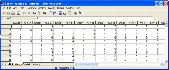
Step 1

STEP2: Click on Analyze followed by selecting correlate -> bivariate. Then move all the variables from ben01 to ben23 in the Variables box. To understand the correlation, click Pearson correlation coefficients in the dialogue box, select a two-tailed test and click on OK.
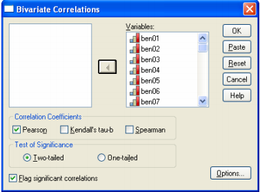
step 2

A glimpse at correlation matrix table
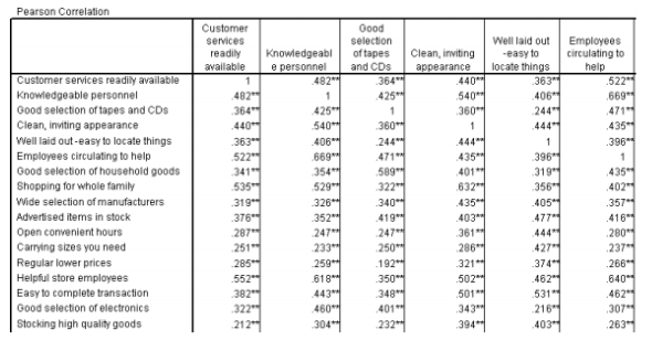
correlation matrix table

NOTE: All correlations are positive and significant at the .01 level and are in the range of 0.3 -0.7. There are definite relations between the factors. Therefore, factor Analysis can be applied in order to reduce the dimensionality of the factors.

STEP3: 

In the third step, click on the Analyze -> Dimension Reduction. Then move all the factor from ben01 to ben23 into the Variables box.
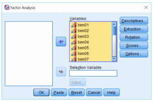
step 3

STEP 4: Click on the Extraction button -> Scree Plot.  

In this step you can either define the number of factors to be computed or leave it blank for SPSS to decide the number of possible factors or you can also select descriptives.
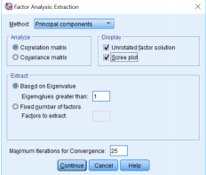
step 4

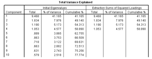
The output table for total variance

output table

The initial eigenvalues has all the 23 variables with the percentage of the variance of all the variables with the cumulative percentage of variance. After running factor analysis in SPSS, we get 4 factors which explain the 58 % of the variance. Any factor which has eigenvalue less >1 would be selected into a particular factor. This is known as eigenvalue greater 1 selection rule.
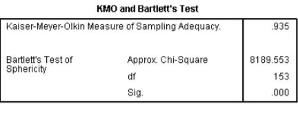
Kaiser-Meyer-Olkin

The Kaiser-Meyer-Olkin is the proportion of examining sufficiency, which ranges somewhere between 0 and 1. However, the estimation of 0.6 is least recommended. Generally, 1>KMO>0.

The sample is sufficient if, KMO is greater than 0.5. 

In the above example, KMO = 0.935 which indicates that the sample is sufficient and we can proceed with the factor analysis. 

Bartlett’s test of sphericity is performed by taking  α = 0.05.  

Here  p-value is .000 less than 0.05, and hence, factor analysis is valid.  

STEP 5 : In this step, select the Dialog Recall tool -> Factor Analysis -> Rotation button 

And select Varimax option button.
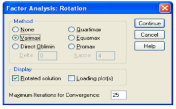
Step 5

STEP 6 : In the final step, click on the continue -> options and then select Sorted by size checkbox followed by selecting Suppress absolute values.
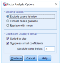
step 6

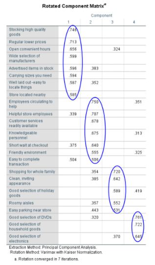
rotated component matrix

This table has unrotated factor loadings which are the correlations between variables and the factors. Here the valid components that we want to retain is selected.

The 4 columns represents that variables are combined into four main factors that explains the variance of the data. 

Factor analysis is mathematically complicated, and the measures applied to determine the number and significance of factors are detailed. It is usually referred to as decrease variables into a factors to save time & help in easy interpretations and is applied to recognise underlying factors. 

Exploring in detail Mann- Whitney U-test which is an alternative to Independent Sample T-test

Independent Sample T-test, popular among various statistical tests, which is used to develop statistical evidence for two populations average is significant or not. The Mann- Whitney U test is the non-parametric equivalent of the one-sample t-test.

The Mann- Whitney U test is the alternative non-parametric test that is used when the assumptions of the selected data are not met. The test uses the ranks of values rather than comparing means. Using ranks only requires that the data should be measured at the ordinal level. However, the main objective or the key purpose of the Mann- Whitney U test is somewhat similar to Independent Sample T-test i.e to provide statistical evidence that the sampled population are different. This test has turned into the most favoured test over that of the Independent Sample T-test. when the assumptions of the Independent Sample T-test holds, it is less likely to detect a location shift in comparison with the test. The test is performed using a two-tail test

The Mann- Whitney U test considers two assumptions for data to be used. The two main assumptions are as follows:-

  • Independence 
  • Should have equal variance.

Note: These assumptions are sufficient for determining if the two populations are different. we take into consideration that the two populations being used should be identical. Considering all assumptions we can use the Mann- Whitney U test on our sample.

Calculating the Mann-Whitney U test 

In order to determine the U test statistics, the mixed set of data is first ordered in ascending order by tied numbers getting a rank similar to the medium position of those numbers in the ordered sequence. The process involves combining all the observations from two samples into one combined sample, also note which observation comes from which samples and then rank all the combined observations from 1 to R1+R2 

Let N: the sum of ranks for the first sample. 

The Mann-Whitney U test statistic is calculated using:

 U = r1 r2 + {r1 (r1 + 1)/2} – N , 

where r1 is first sample  

and r2 is the  second sample

Now, let’s take a simple example :

Sample A

Observation :22 34 45 22 12 19 14

Rank: 15.5 15.5 3.5 12.4 12.5 3.5 2.5

Sample B

Observation :20 14 41 22 12 18 12 13

Rank: 14.5 15.5 3.5 9.4 8.5 6.5 2.5 2.5

Here, T = 82.5,

 R1 = 7, 

 R2 = 8.

Hence, U = (7 * 8) + [{7 * (7+1)}/2] – 82.5 = 8.5

We now compare the calculated U statistic value with the values present in the table. In this example, the values are provided by R1 and R2. By comparing two values we reject or accept the null hypothesis. This method provides a good approximation in the case of large samples. Now that you know everything about this alternative test to the Independent Sample T-test, use it in case of violation of assumptions in correlated-sample situations and perform the test accurately.

Exploring Pearson’s Correlation Coefficient Test to Determine Statistical Relationship Between Two Continuous Variables

Scientific research often involves correlation which generally refers to association or any form of link or correspondence. Correlation is nothing but a statistical approach used to evaluate the linear association between two continuous variables. While several types of statistical tests can be deployed to determine the relationship between two quantitative variables, Pearson’s correlation coefficient is considered as the most reliable test used to measure the continuous variables. 

Pearson’s correlation coefficient is a statistical test that measures the association or relationship  between two continuous variables. Pearson’s correlation coefficient is represented by ‘rho’ and is based on the method of covariance. 

The correlation coefficient or ‘rho’ is the slope of regression line between two variables when they have been standardised by subtracting their means & dividing by their standard deviations. 

Like any other statistical test, Pearson’s correlation coefficient test has a few assumptions including:

  • There is a linear relationship between the variables in the sample which can be assessed by plotting the value of variables on a scatter diagram. 
  • The variables must be normally distributed
  • The variables are either internal or ratio measurements
  • The outliers must be eliminated completely or kept at minimum
  • There exists homoscedasticity of data

Properties of the Pearson’s test 

Limit – Coefficient values range from -1 to +1, where -1 indicates perfect negative relationship and +1 indicates perfect positive relationship and zero indicates absence of relationship.

Symmetric – Correlation of coefficient between two variables is symmetric which simply means that coefficient value between X and Y or Y and X are symmetric.

Pure number – Pure number is independent of unit of measurement. For instance,  if the unit of one variable is in cm and the other is in inches, the Pearson’s correlation coefficient value will remain the same.

When ‘rho’ is utilised as a descriptive statistics, the test doesn’t require any distributional assumptions. When the hypotheses are tested,  it is assumed that the observations are independent and variables are distributed on the basis of bi-variate- normal density function. 

Testing the hypothesis 

Null hypothesis – H0: ρ = 0

Here the population correlation coefficient doesn’t differ significantly from zero. This simply means that there is no significant linear relationship between X and Y.

Alternate hypothesis – Ha: ρ ≠ 0

Here the population correlation coefficient significantly differs from zero. In other words, there is a significant linear relationship between X and Y. 

Method 1 – using the P-value to make a decision 

  • If the p-value is less than the significance level, i.e., alpha= 0.05 then reject the null hypothesis. However, there exists evidence to prove the presence of linear relationship between X and Y as the correlation coefficient is significantly different from zero.
  • If the p-value is equal or greater than the significance level, then the hypothesis shouldn’t be rejected. Here we have sufficient evidence to prove that there is a significant linear relationship 

Method 2 – using a table of critical values  

  • 95% critical values of the sample correlation coefficient table gives an idea whether the computed value of ‘r’ is significant. The critical value can be found using the degrees of freedom (df=n-2).
  •  If ‘r’ value doesn’t lie between the positive and negative critical values, then the correlation coefficient is considered to be significant. 
  • If ‘r’ is significant, then it can be used for line for prediction. However, if ‘r’ is not significant, then you cannot use the line prediction.

The probability of rejecting a false null hypothesis and probability of type-I error is determined by power and alpha. In Pearson’s correlation coefficient test, the value of power & alpha must lie between zero and one. 

Degree of correlation 

The major aspect in Pearson’s correlation coefficient test is the value of correlations. Typically, this value lies between -1and 1. 

Let’s have a detailed look at various types of correlations depending on their value. 

  • Positive correlations – Here the correlation value is positive and the two variables are perfectly positively related. That is, the dots in a scatter line lie on the straight ascending order. 
  • Negative correlation – In this type of correlation the correlation value is -1 and the data points lie on straight descending order. I.e., the variables are linearly negatively related. 
  • Perfect correlation – The correlation is zero and the variables do not have any linear relationship. However, there is a probability of existence of non-linear relationships.

Besides positive, negative and perfect correlation, depending on the value, we have high. Moderate and low degree correlations. 

High degree – Here, the correlation coefficient value lies between  ± 0.50 and ± 1.

Moderate degree – The value lies between  ± 0.30 and ± 0.49.

Low degree – Here, the value lies below + .29.

A glimpse at an example for the Pearson’s correlation coefficient test

10 students held their breath for a minute after breathing normally for 60 seconds and hyperventilating for 60 seconds. Let’s check if there is any association between the two variables ( normal and hyperventilating breathing) for a minimum of 4 students.

Student  A B C D
Normal breathing 55 55 64 64
Hyperventilating breathing  86 90 84 90

According to the graph, there is a linear relationship between the variables. 

Correlation coefficient is one of the most powerful analysis techniques which is purely based on the collected data. Therefore, it is a must to collect accurate data which are capable of providing desired outcomes of the test.

Pursuing doctoral degree in statistics leads in career growth

A Ph.D. in Statistics can lead to better career advancement, especially if you’re a researcher, professor or a government official. A person can take post-graduate studies in statistics to prepare oneself in the business field as well. This degree gives you a deeper understanding of several advanced mathematical areas such as data analysis, probability theory, methodologies, and modeling, just to name a few.

Before you can get a Ph.D. in Statistics, you have to take background courses. Depending on the type of program, you should take up calculus, advanced statistics courses, and linear algebra before enrolling in the doctorate program. Some programs require that you already have an MA degree in Statistics before you can apply for a Ph.D. The program you choose must be based on your research, interest, reputation of the program, budget, and availability.
How to write a statistical dissertation?
Getting things right at the beginning of the process is essential as this will smooth up the process. Correcting mistakes at a later stage is cumbersome and at times impossible. The first and foremost question you should face is the statistical basis of your research paper. The reason for that is quite simple: mistakes in the statistical aspects of the paper will bring more difficulty, distress, disappointment, and failure later on.

While doing the literature review, writing the study proposal, introduction, background and the rest of the dissertation, you will have to include statistical analysis of the data. It is always the statistical significance of the paper that matters. Most importantly, dissertation writing is not a one-man show. Professional dissertation writing involves other disciplines as well, and the assistance that would be the most beneficial for you is that of the statisticians. The involvement of a statistical consultancy company with expert statisticians at the right phase of your dissertation writing will make things easy and help you avoid future worries. Statistical consultancy services offer exclusive statistics consulting and statistics help for doctoral candidates.

Statistics assignments are some of the most challenging types of work that students encounter at school. Today, even during elementary school statistics is introduced, but the level of statistics required to succeed at high school and college is much higher. Students usually find it difficult to write their statistics dissertation on an interesting topic relevant to this subject. They get bored easily with the writing work and thus keep on procrastinating their dissertation writing work. So, in that case, a service that provides expert statistics dissertation help will prove beneficial for the university and college students. Students will have an easy time of dealing with their burdens and frustrations in regards to learning statistics. The tutors ensure every student that they will find the solution for their problems and learn from the basic to the highest level of topics for the subject.