
Statistics, a scientific approach to investigating statistical data, is employed to determine associations among the phenomena to define, predict and control their occurrence.
Factor analysis, known as dimension reduction technique helps to reduce the dimension creating new factors from the old ones by checking the correlations and eigenvalue.
Factor analysis is a helpful technique for researching variable connections for complex ideas, for example, financial status, dietary examples, or mental scales. Based on the correlation matrix of the variables being measured, factor analysis enables scholars to research ideas that are not effectively estimated by combining countless factors into a couple of interpretable basic variables. The sample size should be sufficiently large in order to stabilize the correlations.
Why to use Factor analysis?
Large datasets that consist of several variables can be reduced by observing ‘groups’ of variables into factors and compiles standard variables into descriptive categories. Factor analysis is beneficial for studies that include a few or hundreds of variables, variables from questionnaires, tests which can be reduced to a smaller set, to have an underlying idea, and to help analyses. Other applications include data transformation, mapping, hypothesis-testing and scaling.
Assumptions & requirements of factor analysis
- In order to perform factor analysis its important to run a univariate and multivariate analysis to get the summary of the data. It’s extremely essential to remove all the multivariate and univariate outliers from data. All factor should have at least three or more input variables, though it depends on the statement problem of the research.
- Factors with two variables can also be considered only if input variables are highly correlated with each other but should be analysed with caution.
- The sample size should be sufficiently large more than 300 respondents and variables to examined under factor analysis should be atleast 10 and above.
- As factor analysis measures the linear functions of the variables, it is important to ensure that there is no homoscedasticity within the variables.
- Heterogeneous samples are preferred over homogeneous samples as it lowers the variance and factor loadings of the data.
- All the variables should be linear, ordinal or continuous if not can be transformed into linear variables. Although factor analysis can also be performed on dichotomous variables or categorical variables.
- Missing values should treated or deleted to prevent overestimation.
- The variables should not perfectly correlated to each other. No perfect multicollinearity among the variables of the dataset.
Typically, factor analysis is segregated into two types
- Exploratory factor analysis (EFA) :Takes into account the maximum variance and thereby putting them in factors.
- Confirmatory factor analysis (CFA): Takes into account the common variance and thereby putting them in factors
Components of factor analysis
- Extraction of factors
Factor analysis is theoretical model as it is based on the common factor model. The observed measures are generally affected by the underlying unique and common factors. Maximum likelihood estimates the factor loading of the population.
- Rotation methods
Broadly, there are the orthogonal rotation and oblique rotation. Orthogonal rotation where factors are rotated 90 °, it is believed that the elements are uncorrelated from each other.
- Factor score
A factor score is considered as variable. It tells about the variable load on each factor. One of the methods to generate factor score is called the Bartlett method, which produces unbiased records that are correlated with their factor only .
While there are many tools which can be used to perform factor analysis, the most popular tool among the statisticians is SPSS. Performing factor analysis in SPSS is easier said than done. To understand the steps involved in performing factor analysis, consider the following example.
A researcher wanted to identify the benefits of shopping at the superstore. The researcher took 23 survey questions in order to understand the benefits of shopping at the superstore.
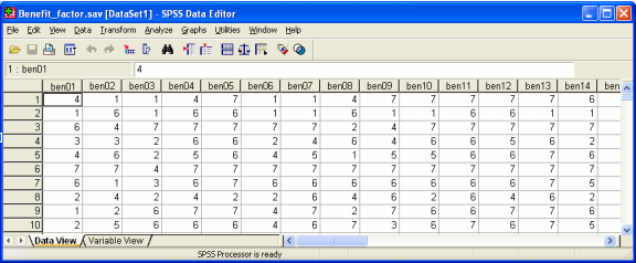
STEP1: The labels were assigned to variables in SPSS in order to perform factor analysis at ease. In this example, the factors are rated on a 1 to 7 scale where 1 implies not important and 7 implies very important. There are a total of 23 factors that have to be examined.
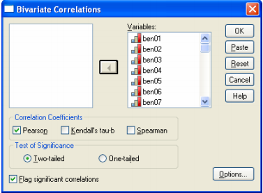
STEP2: Click on Analyze followed by selecting correlate -> bivariate. Then move all the variables from ben01 to ben23 in the Variables box. To understand the correlation, click Pearson correlation coefficients in the dialogue box, select a two-tailed test and click on OK.
A glimpse at correlation matrix table
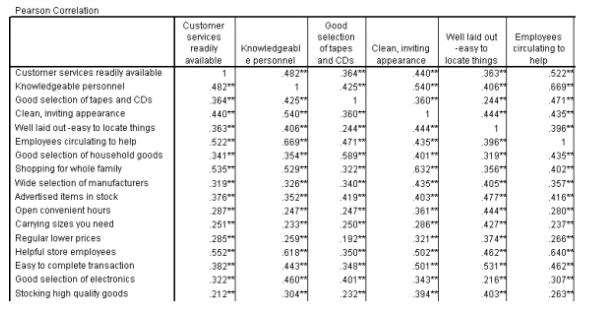
NOTE: All correlations are positive and significant at the .01 level and are in the range of 0.3 -0.7. There are definite relations between the factors. Therefore, factor Analysis can be applied in order to reduce the dimensionality of the factors.
STEP3:
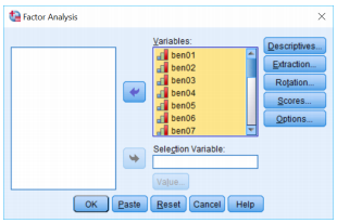
In the third step, click on the Analyze -> Dimension Reduction. Then move all the factor from ben01 to ben23 into the Variables box.
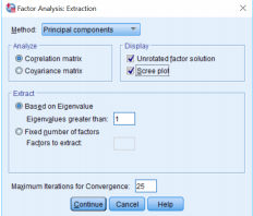
STEP 4: Click on the Extraction button -> Scree Plot.
In this step you can either define the number of factors to be computed or leave it blank for SPSS to decide the number of possible factors or you can also select descriptives.
The output table for total variance
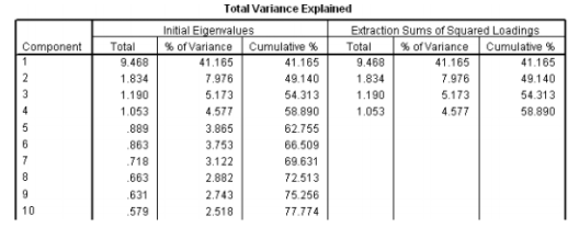
The initial eigenvalues has all the 23 variables with the percentage of the variance of all the variables with the cumulative percentage of variance. After running factor analysis in SPSS, we get 4 factors which explain the 58 % of the variance. Any factor which has eigenvalue less >1 would be selected into a particular factor. This is known as eigenvalue greater 1 selection rule.
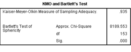
The Kaiser-Meyer-Olkin is the proportion of examining sufficiency, which ranges somewhere between 0 and 1. However, the estimation of 0.6 is least recommended. Generally, 1>KMO>0.
The sample is sufficient if, KMO is greater than 0.5.
In the above example, KMO = 0.935 which indicates that the sample is sufficient and we can proceed with the factor analysis.
Bartlett’s test of sphericity is performed by taking α = 0.05.
Here p-value is .000 less than 0.05, and hence, factor analysis is valid.
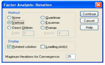
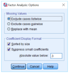
STEP 5 : In this step, select the Dialog Recall tool -> Factor Analysis -> Rotation button
And select Varimax option button.
STEP 6 : In the final step, click on the continue -> options and then select Sorted by size checkbox followed by selecting Suppress absolute values.
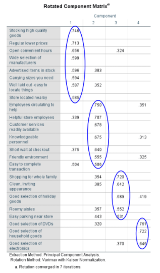
This table has unrotated factor loadings which are the correlations between variables and the factors. Here the valid components that we want to retain is selected.
The 4 columns represents that variables are combined into four main factors that explains the variance of the data.
Factor analysis is mathematically complicated, and the measures applied to determine the number and significance of factors are detailed. It is usually referred to as decrease variables into a factors to save time & help in easy interpretations and is applied to recognise underlying factors.