How to run & interpret repeated measures T-test in SPSS?

Paired sample t-test

A paired sample t-test is used to compare two means where you have two samples in which observations in one sample can be paired with observations in the other sample. Instances, where this might occur, are:

  • After and before observations on the same subjects (e.g. students’ symptomatic test results before and after an appropriate module or course).
  • An association of two different methods of measurement or two different treatments where the computations/methods are applied to the same subjects.

The flow depicts the use of a repeated-measures t-test. There is only one association being inspected at two within-subjects observations or two-time points for a continuous outcome. The assumption of normality of separation records has been met. A repeated-measures t-test is used to assess the change in a continuous outcome at two within-subjects observations or two-time points
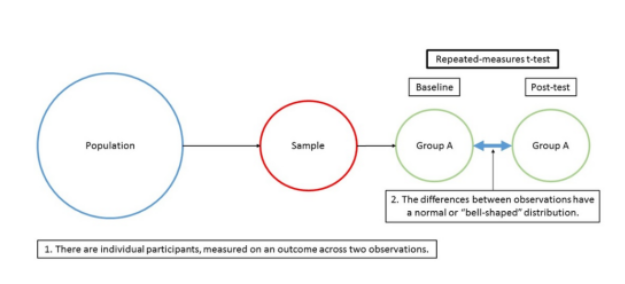
 SPSS help

 ASSUMPTIONS:

The paired sample t-test makes some assumptions. Although t-tests are quite robust, it is a reliable practice to evaluate the degree of deviation from certain assumptions to estimate the essence of the results. The paired sample t-test has four  assumptions:

  • The dependent variable should be continuous (interval/ratio).
  • The observations are independent of one another.
  • The dependent variable should be  normally distributed.
  • There should be no notable outliers in the variances among the two related groups.

Level of Measurement

In paired sample t-test the sample data should be numeric and continuous, as it should be normally distributed. Continuous data can take on any value within a range . The contrast of constant data is discrete data, which can only take on a few value .Occasionally, discrete data can be used to approximate a continuous scale example likert scale.

Independence

Independence is usually not testable but can be reasonably assumed if the data collection process was random without replacement. Example, it is good enough to assume that the participating patients are independent of one another.

 Normality

To test the presumption of normality, a variety of methods are available.  Real-world data are rarely perfectly normal, so this assumption can be regarded as fairly met if the state looks nearly symmetric and bell-shaped.

Example

A group of Sports students (n = 20) is picked from the population to examine whether a 19-week preparation program improves its standing high jump performance. This method is used to test whether this training increases performance, the students are tested for their long jump performance before they begin a training program and then at the end of the programme (i.e., the dependent variable is “standing high jump performance”, and the two similar groups are the standing high jump values “before” and “after” the 19-week training program).

Test Procedure in SPSS Statistics

The six steps below explain to you how to analyze your data using a dependent t-test in SPSS Statistics Assumptions, should not be outraged. Following the six steps, the interpretation of the results is also commuted depending on the data analysis.

  1. Click Analyze 

> Compare Means

 > Paired-Samples T Test… on the top menu, 
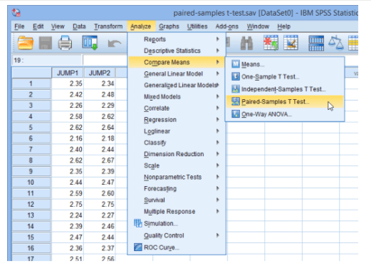
spss consultant

  1. You will be shown with the Paired-Samples T Test dialogue box, as explained here:
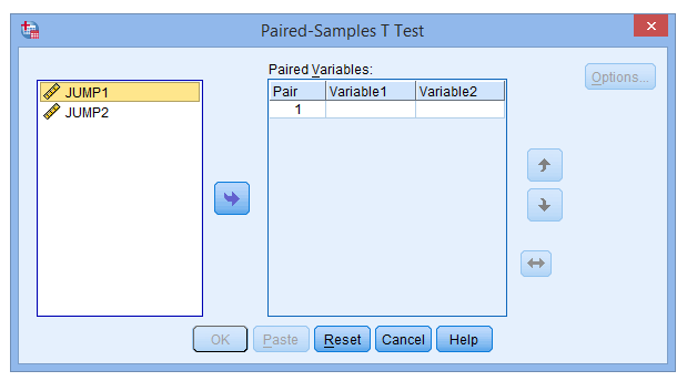
 spss help services

  1. Assign the variables JUMP1 and JUMP2 within the paired box. There are two methods to do this: 

(1) click on both variables whilst bringing down the shift key and then pressing the button

 (2) drag-and-drop each variable individually into the boxes.
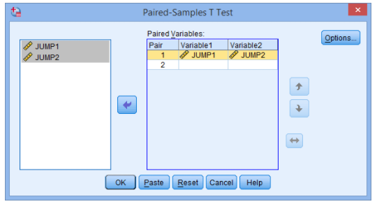
T test help

  1. If you want to adjust the confidence level limits or eliminate cases, click on the options button. After performing the Paired-Samples T-Test: Options dialogue box, as explained here:
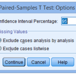
 

5.Click the continue button. You will be returned to the Paired-Samples T Test dialogue box

6.Click the OK button.

INTERPRETATIONS:

PSS Statistics generates three tables in the Output Viewer under the title “T-Test”,look at two tables: the Paired Samples Statistics table and the Paired Samples Test table.

Paired Sample Statistics Table

The initial table, titled Paired Samples Statistics, is where SPSS Statistics has generated detailed statistics for your variables. You could use the results here to describe the features of the first and second jumps in the write up
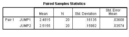
 paired sample statistics

 Paired Samples Test Table

The Paired Samples Test table is wherever the results of the dependent t-test are presented. A lot of information is displayed here and it is essential to identify that this information refers to the variations between the two jumps.  paired sample test
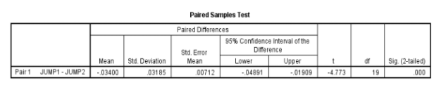
 When drafting up the results of your t-test you need to report whether or not the test was significant developing this formula:

 t (df) = t value,

 p = p-value

For this particular example, we have found that the t-test is significant as the p-value is less than 0.05.

Results : t(19) = -4.773, p < 0.001

When interpreting we need to use information from both descriptive and inferential statistics in your output.

 1: State the pattern of your data using the means and standard deviations from the first output table.

 Results showed participants made a larger amount of ‘JUMP2’  (mean=2.51 , SD = 1.61) than for JUMP1 (mean = 2.48, SD = 0.159).

2: Report whether or not this difference is significant: A repeated-measures t-test found this difference to be significant,

 t(19) = -4.773, p < 0.001. ·

3: Finally, you need to put this information together to understand and compile what we have found in terms of your hypothesis. therefore, we can reject the null hypothesis and accept the alternative hypothesis.
Spoiler alert ahead: Great tips for conducting factor analysis using SPSS

Statistics, a scientific approach to investigating statistical data, is employed to determine associations among the phenomena to define, predict and control their occurrence.

Factor analysis, known as dimension reduction technique helps to reduce the dimension creating new factors from the old ones by checking the correlations and eigenvalue. 

Factor analysis is a helpful technique for researching variable connections for complex ideas, for example, financial status, dietary examples, or mental scales. Based on the correlation matrix of the variables being measured, factor analysis enables scholars to research ideas that are not effectively estimated by combining countless factors into a couple of interpretable basic variables. The sample size should be sufficiently large in order to stabilize the correlations. 

Why to use Factor analysis? 

Large datasets that consist of several variables can be reduced by observing ‘groups’ of variables into factors and compiles standard variables into descriptive categories. Factor analysis is beneficial for studies that include a few or hundreds of variables, variables from questionnaires, tests which can be reduced to a smaller set, to have an underlying idea, and to help analyses. Other applications include data transformation, mapping, hypothesis-testing and scaling.

Assumptions & requirements of factor analysis 

  • In order to perform factor analysis its important to run a univariate and multivariate analysis to get the summary of the data. It’s extremely essential to remove all the multivariate and univariate outliers from data. All factor should have at least three or more input variables, though it depends on the statement problem of the research. 
  • Factors with two variables can also be considered only if input variables are highly correlated with each other but should be analysed with caution. 
  • The sample size should be sufficiently large more than 300 respondents and variables to examined under factor analysis should be atleast 10 and above.
  • As factor analysis measures the linear functions of the variables, it is important to ensure that there is no homoscedasticity within the variables.
  • Heterogeneous samples are preferred over homogeneous samples as it lowers the variance and factor loadings of the data.
  • All the variables should be linear, ordinal or continuous if not can be transformed into linear variables. Although factor analysis can also be performed on dichotomous variables or categorical variables.
  • Missing values should treated or deleted to prevent overestimation.
  • The variables should not perfectly correlated to each other. No perfect multicollinearity among the variables of the dataset. 

Typically, factor analysis is segregated into two types

  • Exploratory factor analysis (EFA) :Takes into account the maximum variance and thereby putting them in factors. 

Components of factor analysis

  • Extraction of factors 

Factor analysis is theoretical model as it is based on the common factor model. The observed measures are generally affected by the underlying unique and common factors. Maximum likelihood estimates the factor loading of the population. 

  • Rotation methods 

Broadly, there are the orthogonal rotation and oblique rotation. Orthogonal rotation where factors are rotated 90 °, it is believed that the elements are uncorrelated from each other.

  • Factor score 

A factor score is considered as variable. It tells about the variable load on each factor. One of the methods to generate factor score is called the Bartlett method, which produces unbiased records that are correlated with their factor only . 

While there are many tools which can be used to perform factor analysis, the most popular tool among the statisticians is SPSS. Performing factor analysis in SPSS is easier said than done. To understand the steps involved in performing factor analysis, consider the following example.  

A researcher wanted to identify the benefits of shopping at the superstore. The researcher took 23 survey questions in order to understand the benefits of shopping at the superstore. 

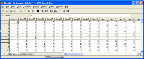
STEP1: The labels were assigned to variables in SPSS in order to perform factor analysis at ease. In this example, the factors are rated on a 1 to 7 scale where 1 implies not important and 7 implies very important. There are a total of 23 factors that have to be examined.

Step 1

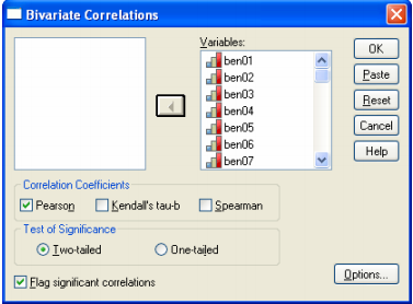
STEP2: Click on Analyze followed by selecting correlate -> bivariate. Then move all the variables from ben01 to ben23 in the Variables box. To understand the correlation, click Pearson correlation coefficients in the dialogue box, select a two-tailed test and click on OK.

step 2

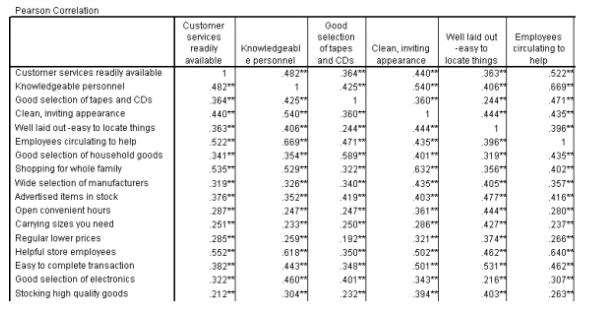
A glimpse at correlation matrix table

correlation matrix table

NOTE: All correlations are positive and significant at the .01 level and are in the range of 0.3 -0.7. There are definite relations between the factors. Therefore, factor Analysis can be applied in order to reduce the dimensionality of the factors.

STEP3: 

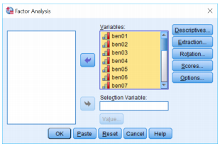
In the third step, click on the Analyze -> Dimension Reduction. Then move all the factor from ben01 to ben23 into the Variables box.

step 3

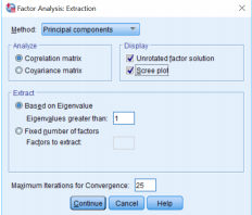
STEP 4: Click on the Extraction button -> Scree Plot.  

In this step you can either define the number of factors to be computed or leave it blank for SPSS to decide the number of possible factors or you can also select descriptives.

step 4

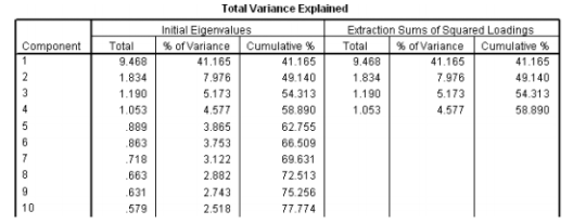
The output table for total variance

output table

The initial eigenvalues has all the 23 variables with the percentage of the variance of all the variables with the cumulative percentage of variance. After running factor analysis in SPSS, we get 4 factors which explain the 58 % of the variance. Any factor which has eigenvalue less >1 would be selected into a particular factor. This is known as eigenvalue greater 1 selection rule.

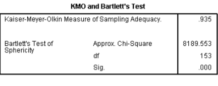
Kaiser-Meyer-Olkin

The Kaiser-Meyer-Olkin is the proportion of examining sufficiency, which ranges somewhere between 0 and 1. However, the estimation of 0.6 is least recommended. Generally, 1>KMO>0.

The sample is sufficient if, KMO is greater than 0.5. 

In the above example, KMO = 0.935 which indicates that the sample is sufficient and we can proceed with the factor analysis. 

Bartlett’s test of sphericity is performed by taking  α = 0.05.  

Here  p-value is .000 less than 0.05, and hence, factor analysis is valid.  

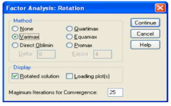
STEP 5 : In this step, select the Dialog Recall tool -> Factor Analysis -> Rotation button 

And select Varimax option button.

Step 5

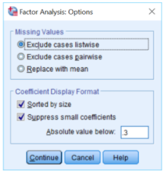
STEP 6 : In the final step, click on the continue -> options and then select Sorted by size checkbox followed by selecting Suppress absolute values.

step 6

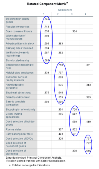
rotated component matrix

This table has unrotated factor loadings which are the correlations between variables and the factors. Here the valid components that we want to retain is selected.

The 4 columns represents that variables are combined into four main factors that explains the variance of the data. 

Factor analysis is mathematically complicated, and the measures applied to determine the number and significance of factors are detailed. It is usually referred to as decrease variables into a factors to save time & help in easy interpretations and is applied to recognise underlying factors. 

Know the Difference: Parametric Test and Non-Parametric Test in Statistics

Statistical tests are mind bogglers! Collection, organisation, interpretation and analysis of data and results constitutes an integral part of statistics. Statistical tests, are basically the medium through which we can approximate solutions when the processes are highly complex or unknown in their true forms.

Statistical tests are classified into

  1. parametric test, and
  2. non parametric test

Parametric test-

Parametric test (conventional statistical procedure) are suitable for normally distributed data. The majority of elementary statistical methods are parametric, and parametric tests generally have higher statistical power.

  1.  In the parametric test, the test statistic is based on distribution.
  2.  The measurement of variables of interest is done on interval or ratio level.
  3.  In general, measure of central tendency in the parametric test is mean.
  4.  Parametric test can be applied only for the variables.
  5.  This test provides you with complete information about the population.

Parametric Test for Independent Measures Between Two Groups: T-test- A t-test is used to compare between the means of two data sets, when the data is normally distributed. Here, the two groups of data must be independent from one another.

Parametric correlation test: Pearson test – A common parametric method of measuring correlation between two variables is the Pearson Product-Moment Correlation. In this test, the variables should be normally distributed.

Why should you use parametric test?

  1.  Parametric tests can perform well with skewed and non normal distributions
  2.  Parametric tests can perform well when the spread of each group is different
  3.  Parametric tests usually have more statistical power than nonparametric tests

Non parametric test

Non parametric test (distribution free test), does not assume anything about the underlying distribution. Non parametric tests are used when the data isn’t normal.

  1.  In the case of non parametric test, the test statistic is arbitrary.
  2.  The variable of interest are measured on nominal or ordinal scale.
  3.  The measure of central tendency is median in case of non parametric test.
  4.  Non parametric test doesn’t consist any information regarding the population.
  5.  This test can be applied to both variables as well as attributes.

Non Parametric Test for Independent Measures Between Two Groups: Mann-whitney test-  This test is used to compare the means between two groups of ordinal data.

Non parametric correlation test: Spearman test- This test is used when data are ordinal rather than interval. This test works the same as the Pearson Correlation test, but the data here must first be ranked.

Reasons to use non parametric test

  1. Your area of study is better represented by the median
  2. Your sample size is too small to run a parametric test
  3. Your have ordinal/ ranked data or outliers that cannot be removed

Lastly, to use parametric test or nonparametric test often depends on whether the mean or median more accurately represents the center of the data set’s distribution. If the mean represents the center of the distribution of your data, and the sample size is large enough, use  parametric test and if the median represents the center of the distribution of your data, use non parametric test.


Understanding SPSS Variables: Format, Type and More

If you understand SPSS variable formats and types, it will help you in getting things done accurately and quickly. Learn the format and type of SPSS variables and get in control of your data.

Ascertaining SPSS Variable Formats

SPSS differentiates write and print formats. SPSS variable format comprises of two parts. The format family is indicated by one or more letters. Most the letters speak to themselves, excluding the first two variables:

  • F (Fortran), indicating a standard numeric variable.
  • A (Alphanumeric), the common format for string variables.

Formats end with numbers, which indicate the number of characters which is required to be shown. If you find a period, the number which is present after the period represents the number of decimal places which needs to be displayed.

SPSS Variable Types

SSPS has two variable types, namely numeric and string. String variables may contain numbers, letters and other characters. Numeric variables may include just numbers. The difference between string and numeric variables is crucial due to the fact that variable type dictates what you can or cannot do with a variable.

  • You can use string functions like concatenating with string variables and taking substrings but not with numeric variables.
  • You can do calculations with the use of numeric variables but not with string variables.

In SPSS, there are no other variable types other than numeric and string. But numeric variables have varied distinct formats that are often confused with variable types.

Numeric Type

Numeric variables contain values that are in number form, like in scientific notation or standard format.

For instance: Counts (like number of free throws given in each game) are a numeric variable containing zero decimal places. Some of the mathematical calculations are allowed when applied for counting variables (like standard and mean deviation), but some statistical processes are excluded (like linear regression).

For instance: Continuous variables that can easily take any number in a range (like blood pressure, weight, height etc.) can be regarded as numeric variables. The researcher is allowed to select as many or few decimal places as they think is required. This type of variable is utilized in calculations, like computing standard and average deviations of heights.

String Variables

Also known as character variables or alphanumeric variables, string variables have values that are considered as text. This infers that the values of string variables may contain symbols, letters or numbers. The string values that are missing may appear blank.

The Need of SPSS for a Successful Dissertation

Most candidates of US who are in the process of completing a dissertation or master’s thesis presently or in future have a common question to ask that is whether it is necessary to learn SPSS (Statistical Package for Social Sciences) for the preparation of a successful dissertation project. At some point of time it is necessary to know SPSS for the benefit of your project work. So many graduate and doctoral programs focused mainly on research related work exposes their students to the need for learning SPSS and its proper application in the dissertation process. The SPSS statistics software has an important application in the dissertation work and researchers use it to perform statistical analysis of their research work. The software can import any form of dissertation data for analysis purpose, to generate charts, tabulated data and descriptive statistics as well.

Learning the use of SPSS
There are various consulting firms and companies which helps you to learn SPSS so that you can benefit from it in your dissertations. Although apparently it might seem quite easy to use the features of this software but gradually you will realize the need for an expert guidance to operate the software properly. There are various steps which each candidate must learn to successfully avail the benefits of the SPSS statistical package. The first thing is to learn the method of entering dissertation data in SPSS, the next step being the process of entering and labeling dissertation variables in SPSS. The final stage is the way you should read the dissertation statistical analyses prepared in SPSS. All these take a considerable amount of time and every candidate must learn it in depth to smoothly glide through the process of dissertation work. Each and every step and the sub steps within them are equally important to carry out dissertations in SPSS. There are also various online consultation services which provide the facility of teaching SPSS where candidates all over the world can have the privilege of learning this easy-to-use statistical package.

Benefits of outsourcing such task
Many US doctoral candidates have a dilemma in their mind whether to learn the mechanism of SPSS or outsource such task to a consulting firm. Though some people may be of the opinion that learning to use SPSS should be beneficial as it is only the individual who knows best how to present their work but from a practical viewpoint it is both safe and convenient to outsource the task of SPSS to a consulting firm. There are several reasons for this; firstly you won’t need to spend your valuable time learning SPSS for your research work and fully concentrate on the dissertation you are preparing. Moreover you can avail the services of expert professionals to carry out the SPSS task for you and make your dissertation more presentable and acceptable. So it should be sensible to outsource such task to companies like Statistics Consultation rather than spending 500 hours in learning and mastering such a software which would be of no use after you finish your research work.